What ESA announced this week

On 31 July 2026, the European Space Agency published that the HydroGNSS Scout mission has completed commissioning, entered full scientific operations, and that HydroGNSS data are freely available to users worldwide. The primary write-up is ESA’s own article, “HydroGNSS data open for new insights into Earth's water”.

For GIS developers, analysts, journalists, civic technologists, and web-mapping practitioners, the useful story is not another “new satellite” headline. It is a concrete access and geometry problem: what variables exist, how registration works, what spatial character the products have, and how to fold derived features into ordinary vector and web workflows without pretending the mission ships browser-ready GeoJSON.

This checklist sticks to what ESA’s announcement supports, flags what still needs product-document verification, and sketches a pipeline you can run with desktop GIS, notebooks, and a browser editor once you hold derived vectors in hand.

Mission basics in plain language

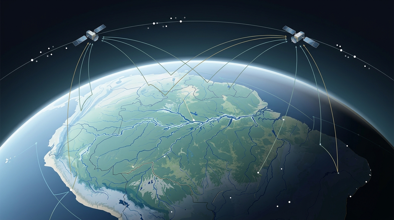
HydroGNSS is a two-satellite Scout mission. Per ESA, the pair launched in November 2025 and measures Earth using GNSS Reflectometry (GNSS-R).

GNSS-R is not optical imagery and not a classic active radar sounder in the newsroom sense. Navigation satellites (for example GPS and Galileo) continuously broadcast L-band signals. HydroGNSS compares signals reflected from Earth’s surface with direct signals. From those comparisons, processing chains estimate hydrological and vegetation-related quantities.

That distinction matters for map design:

You should expect science products with mission-specific sampling, not a daily global “pretty picture” layer that drops straight into a basemap slider.
L-band reflectometry can be valuable when clouds, night, or vegetation structure limit optical methods—but product handbooks, uncertainty fields, and validation literature still govern whether a given pixel or sample is fit for a public map.

ESA names several derived hydrological variables associated with the mission and its processing partners (SSTL with scientific collaborators), including:

Soil moisture
Inundation and wetlands
Freeze–thaw dynamics
Above-ground biomass / vegetation-related products

Treat that list as the announced science themes, not as a guarantee that every theme is already a polished, analysis-ready layer for every region and date.

Geometry you should plan for: tracks, not wall-to-wall wallpaper

One concrete geometric detail in ESA’s piece is especially important for web mappers. ESA describes coherent-channel measurements used to identify water surfaces as being collected along satellite tracks at 300 m resolution, with observations from both satellites combined over time for fuller coverage.

Implications for cartography and data engineering:

Point or segment overlays often fit better than country-scale choropleths. Track-wise samples naturally become points, multipoints, or short line segments with time and quality attributes—not seamless administrative fills.
Time stacking is part of the product story. “Fuller coverage” in the announcement is framed as combining passes over time, so a single-day snapshot may look sparse even when the multi-week composite is useful.
Do not generalize 300 m to every variable. ESA’s 300 m language in the announcement is tied to the coherent-channel water-surface illustration path. Soil moisture, freeze–thaw, and biomass products may differ in posting, footprint, and recommended scale. Confirm each product family in the official docs after you register.
Browser maps will usually show derived vectors. Upstream work (subset, quality filter, optional rasterization or vectorization) happens in analysis tools; the web layer is the communicate-and-QA step.

If your mental model is “global GeoTIFF every morning → COG → XYZ tiles,” pause. HydroGNSS may still participate in raster workflows, but the public announcement’s clearest geometry hook is along-track sampling—plan overlays accordingly until handbooks say otherwise.

Access path: free worldwide, not anonymous bulk download

ESA’s wording is precise enough to prevent a common mistake:

Freely available worldwide does not automatically mean “no account, no forms, CDN tarball.”
ESA directs users to obtain product information and register for access through the SSTL HydroGNSS website.

Before you promise a newsroom or civic partner a one-click open dataset, verify on the live SSTL portal:

Whether access is immediate after registration or reviewed
Identity, affiliation, or use-case fields
Quotas, rate limits, or redistributions rules
Exact license text for derived maps and republished subsets
On-disk or API forms (do not assume NetCDF, GeoTIFF, COG, STAC, or GeoJSON from the ESA news page alone)
CRS, time stamps, latency from acquisition to release, and quality-flag definitions

Until those details are confirmed in primary product documentation, keep public language at the level ESA supports: operations have started; data are openly offered; registration is via SSTL.

A practical week-one pipeline for web mappers

The goal is a defensible overlay, not a black-box “satellite truth” layer. A sober sequence looks like this.

1. Register and read before you script

Create the SSTL HydroGNSS access path ESA points to. Download the product guide / ATBD / format notes for the variable you actually need (wetlands vs soil moisture vs freeze–thaw are different cartographic animals). Note version strings and any DOI or citation requirements.

2. Define an area and a question that matches the sampling

Good fit examples:

“Where do recent coherent water-surface indications fall along tracks crossing this floodplain?”
“How do freeze–thaw flags line up with road-closure reports this week?”
“Which field sites show soil-moisture anomalies worth a second look against local gauges?”

Weaker fit examples:

Seamless county choropleths from a single sparse pass
Legal property boundaries or parcel-level insurance decisions from unvalidated samples
Nightly global “wetness index” basemaps without documented compositing rules

3. Subset upstream, then QA

Use your normal EO stack—GDAL/rasterio, xarray, QGIS, or mission-provided tools—to clip to the AOI, filter on quality flags, and keep provenance columns (acquisition time, satellite id, product version, uncertainty if present). Discard or style differently samples that fail QA rather than silently mapping them as equal facts.

4. Derive vectors intentionally

Depending on the product and your question:

Track points with soil-moisture or freeze–thaw attributes for sparklines and hover cards
Line segments along specular tracks for “pass coverage” diagrams
Polygons only after a documented classification or threshold step (for example wetland indication regions), with the threshold and date range in the layer metadata

Keep attribute names boring and explicit: obs_time, variable, value, unit, quality, source_product, notes.

5. Validate against something local

Before publication:

Cross-check a handful of points against gauges, flood bulletins, land-cover maps, or trusted optical/SAR context layers
Record disagreements; do not only keep confirming samples
State residual uncertainty in the legend or method note

6. Hand off to web interchange formats

Once you have clean vectors, ordinary web tooling applies. Export GeoJSON (or KML / zipped Shapefile / CSV points) for newsroom graphics, civic dashboards, or collaborative QA. Browser editors such as GeoJSON Cloud are relevant at this overlay and interchange step: open the derived features, inspect properties, fix obvious geometry or attribute issues, and export a shareable GeoJSON. They are not a HydroGNSS archive, GNSS-R processor, or substitute for SSTL/ESA product access.

If partners send you tabular site lists, convert carefully (CSV with lon/lat → points) and keep the HydroGNSS provenance fields intact so editors downstream can see what the dots actually mean.

Use cases that stay honest

Journalists can use track-wise inundation or soil-moisture context beside river-gauge charts and ground photos—labeled as mission-derived indications, with date ranges and registration/source links—not as standalone proof of a flood crest at a street address.

Civic technologists can prototype drought or freeze–thaw dashboards that combine HydroGNSS-derived site markers with local open data (road conditions, agricultural advisories). Start with pilot AOIs and documented refresh cadence.

GIS developers should wrap access assumptions behind config (endpoint, credentials, product version) and design schemas that survive product version bumps. Prefer reproducible notebooks that emit both a QA report and a web GeoJSON.

Analysts can treat early open data as a chance to build validation sets and uncertainty visualizations, not only polished cartography.

In all cases, ESA’s climate and water framing is agency science communication. Educational maps should describe observables and methods, not guaranteed policy or impact outcomes.

What not to claim yet

Until a human opens the live SSTL documentation and sample files, avoid asserting:

Specific file formats, STAC availability, or public S3-style bulk mirrors
Universal 300 m resolution across all variables
Near-real-time latency numbers
Native GeoJSON delivery from the mission
Fitness for regulatory, insurance, or life-safety decisions without independent validation

Secondary social roundups that bundle HydroGNSS with unrelated releases are useful only as awareness; they are not substitutes for the ESA primary article or SSTL product pages.

Bottom line

HydroGNSS’s open-data milestone is timely because operations plus worldwide free access lowers the barrier to experimentation—not because browser maps suddenly understand GNSS-R natively. Register via the SSTL path ESA names, learn each product’s sampling and quality model, derive vectors that match the science, and only then push GeoJSON overlays onto the web with clear uncertainty labels.

That workflow keeps the excitement proportional to the evidence and keeps your maps usable when the next product version lands.

Sources and further reading

European Space Agency — HydroGNSS data open for new insights into Earth's water (31 July 2026)
Follow ESA’s pointer to the SSTL HydroGNSS site for registration, product lists, and format documentation (confirm details on the live portal; not fully specified in the ESA news article alone)